Before I started working as a software engineer, I had majored in Energy Engineering, and I particularly liked the field of Energy Modeling. From Wikipedia:
Energy modeling is the process of building computer models of energy systems in order to analyze them. Such models often employ scenario analysis to investigate different assumptions about the technical and economic conditions at play.
Researchers in this field try to answer questions such as:
- How much electricity will South America need in 2040? Can it be realistically achieved with 25% of it generated from renewable sources? What about 50%? 80%?
- What would be the cost of achieving full access to electricity in Burkina Faso?
- What would be the impact of introducing clean cookstoves on the economics of families in rural Kenya? – this particular question was the subject of my Master’s thesis.
Most of the energy modeling work I am familiar with is done at the division of Energy Systems Analysis (dESA) at the Royal Institute of Technology (KTH) in Stockholm. dESA is an academic institute working with energy models ranging from the very local (villages) to the very global (continents). They partner with institutions like the UN and the World Bank and contribute to reports such as the World Energy Outlook, which many consider being the most important reference when it comes to predicting future energy usage.
OSeMOSYS at dESA
While simple energy systems can be modeled using Excel spreadsheets, more complex ones require specialized software.
Enter OSeMOSYS, an open source energy modeling software created at dESA. It allows researchers to model large-scale energy systems such as the electricity generation of a whole continent.
Once the model created, OSeMOSYS translates it to a mathematical model consisting of linear equations. Finding a solution for these kinds of models is the field of linear optimization and is infamous for being computationally very intensive1 – large models at dESA can sometimes require more than 10 hours to run.2
Issues with today’s setup
To run their simulations, dESA researchers use either their personal computer or one of the high powered desktop workstations available in the lab.
I sent out a survey to the department to get more information about their day-to-day workflow. Some highlights:
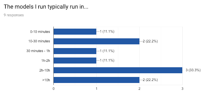 Models duration
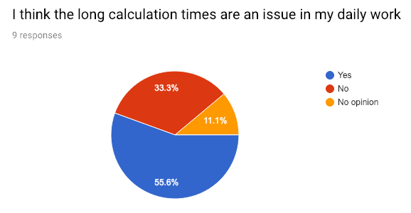 Calculation times are a problem
More than half the surveyed researchers think that the long calculation times are frustrating. That should’t come as a surprise, as the drawbacks of long feedback loops are well known – context switching alone is a major productivity sink. And because the simulations often take up 100% of the available CPU and memory on the machines:
- The computer running the simulation becomes very slow and basically unusable during the time the model is running.
- A given computer can only run one simulation at a time.
That got me thinking… what if a researcher could spin up a fast machine with plenty of CPU and memory, use it to solve their model and then throw it away?
Enter The Cloud
If we were able to run a typical OsMOSYS workload on a computer in the cloud, we would make it possible to:
- make computations faster, as the machine would be 100% dedicated to solving the problem, with no significant overhead coming from the OS and other running programs
- simultaneously run multiple models
- free up the desktop workstations to do more work
So let’s try to do just that!
Proof of concept
We’ll use AWS EC2 to test-drive this idea. EC2 lets you create (“provision” in tech jargon) virtual machines in Amazon’s data centers almost instantly. There are different types of machines (“instances”) we can chose from, each with different characteristics. Some have large hard drives, some have more memory, and some are especially tailored towards computationally heavy tasks. The last kind is the one we are interested in: the Compute Optimized c5 instance types. We can for example get a 16-core, 32Gb memory instance (c5.4xlarge) and get billed for it on a per-second basis.
Setup
Using the AWS web interface, we can create an instance without leaving the browser. But spinning up the machine is just the beginning: once the machine is created and online we get an ip address we can connect to using ssh, and then:
- Setup all the dependencies needed to perform the calculations, for example:
- Compiling GLPK from source (it is not available as a pre-packaged packet on the Amazon Linux AMI)
- Downloading and installing a demo version of CPLEX
- Download the model files
- Monitor the solver while it’s running
- Upload the result and log files after a solution is found
Hopefully thanks to EC2’s AMI feature, the first step only has to be done once. After that we can create an image and use it to spawn new instances with a pre-installed GLPK and CPLEX.
Since this is a proof of concept, for steps 2 and 4 we can just upload the model files to a bucket on AWS S3 (AWS file storage service) with the right permissions (granted through AWS IAM, the access management service) and call it a day.
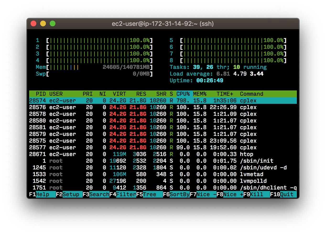
We can then run the solver in a tmux session so we don’t have to stay connected to the machine, and monitor it from time to time using htop.
Results
I used the SAMBA model for my tests3. It is an energy model of the electricity supply of South America and is one of the most computationally heavy models dESA is working with. It usually takes 4 hours using the CPLEX solver.
The first step is to convert the model files to a format that CPLEX can read using glpsol:
~$ > glpsol -m my_model.txt -d my_data.txt --wlp input.lp --check
[...]
Finished in 3226.515 seconds with exit status 0 (successful)
That’s 53 minutes just to generate the input file! Talk about a heavy model :)
Once we have the input file, we use CPLEX to solve it:
~$ > cplex -c "read input.lp" "optimize" "write output.sol"
[...]
Solution time = 2913.96 sec.  Iterations = 998341 (54)
Deterministic time = 1175541.31 ticks  (403.42 ticks/sec)
That’s another 2913 seconds, i.e. 48 minutes to solve the model.
That puts the total solving time at 1h40. Not bad going from a 4h baseline! It’s a 2.3 times faster than running it on a workstation.
Conclusions
We now have a way to perform OsEMOSYS calculations in the cloud. Not only can this speed up energy simulations by at least a factor of 2, but it can also allow researchers to work on multiple models in parallel.
However, the solution as presented in this article still requires too much manual setup to be viable for everyday use. It requires for example prior knowledge of the AWS ecosystem and experience with unix-like systems and the command line.
A logical next step would be to automate the process even further, so that the researchers don’t have to worry about the technical details of how their models get run. Maybe through a web UI?
On a more general note, this experiment got me thinking about the state of software engineering in academia. Having been immersed in both worlds, I feel like academia can (and needs to) learn from software engineering as an industry and vice versa. How can we allow for these worlds to collide and benefit from each other?
If that’s something that you are interested in, I’ll be happy to discuss it further! Send me an email: youssef [at] yboulkaid.com
Nerdy notes
vCPU settings:
When creating an instance EC2 lets us choose how many threads the CPU will have, by tweaking the number of cores and threads per core.
This setting depends on how parallelizable the task we want to run is. After some trial and error I found that:
- GLPK is purely single-threaded and will not benefit from more cores at all.
- While CPLEX can run on multiple threads, it is much more inefficient than when running on a lower number of cores.
So for our use case, the lower number of vCPUs is, the better. But it’s fun to look at a window like this:
Choosing the right instance type:
AWS provides several tiers of performance-optimized instances, ranging from c5.large with 2vCPUs and 4Gb of RAM to the monster that is the c5.18xlarge, with up to 72 vCPUs and a whopping 144Gb of RAM!
We already know that 2vCPUs will be enough for us. Lowering the number of vCPUs on a machine will not “concentrate” the power into one vCPU, as all vCPUs correspond to the same unit:
Each vCPU is a thread of either an Intel Xeon core or an AMD EPYC core
So the limiting factor will only be the amount of RAM needed. CPLEX can be quite RAM demanding, and I have had machines crashing because they were running out of memory. The minimum amount of RAM that would keep a machine from crashing under the SAMBA workload was 32Gb, so that’s what I used (c5.4xlarge).
The power of gzip
The ouput files from calculation results can be (very) large! For example, the output of the SAMBA model is a text file with a bit more than 11.7 million lines. That amounts to 1.58Gb on disk!
However, they’re not very dense in actual information, as most of it is redundant:
  <variable name="WBResidualCapacity(REGION1,VE_RI,2052)" index="6025027" status="BS" value="8.8499999999999996" reducedCost="0"/>
  <variable name="WBResidualCapacity(REGION1,VE_RI,2053)" index="6025028" status="BS" value="8.8499999999999996" reducedCost="0"/>
  <variable name="WBResidualCapacity(REGION1,VE_RI,2054)" index="6025029" status="BS" value="8.8499999999999996" reducedCost="0"/>
  <variable name="WBResidualCapacity(REGION1,VE_RI,2055)" index="6025030" status="BS" value="8.8499999999999996" reducedCost="0"/>
  <variable name="WBResidualCapacity(REGION1,VE_RI,2056)" index="6025031" status="BS" value="8.8499999999999996" reducedCost="0"/>
  <variable name="WBResidualCapacity(REGION1,VE_RI,2057)" index="6025032" status="BS" value="8.8499999999999996" reducedCost="0"/>
  <variable name="WBResidualCapacity(REGION1,VE_RI,2058)" index="6025033" status="BS" value="8.8499999999999996" reducedCost="0"/>
  <variable name="WBResidualCapacity(REGION1,VE_RI,2059)" index="6025034" status="BS" value="8.8499999999999996" reducedCost="0"/>
  <variable name="WBResidualCapacity(REGION1,VE_RI,2060)" index="6025035" status="BS" value="8.8499999999999996" reducedCost="0"/>
  <variable name="WBResidualCapacity(REGION1,VE_RI,2061)" index="6025036" status="BS" value="8.8499999999999996" reducedCost="0"/>
  <variable name="WBResidualCapacity(REGION1,VE_RI,2062)" index="6025037" status="BS" value="8.8499999999999996" reducedCost="0"/>
  <variable name="WBResidualCapacity(REGION1,VE_RI,2063)" index="6025038" status="BS" value="8.8499999999999996" reducedCost="0"/>
That makes those files the perfect candidates for compression. A simple gzip compresses the file to only 88Mb, which is only 5.5% of the original file size. Pretty impressive! :)
-
The problem of linear programming is NP-hard is still an area of active research. ↩
-
Simple problems are solved using the open source GNU Linear Programming Kit (GLPK). However, for more complex problems the task is too heavy for GLPK and dESA uses commercial software like IBM’s CPLEX optimizer to find a solution in a reasonable amount of time. ↩
-
The simulations were run with the
OSeMOSYS_2013_05_10.txtmodel file andSAMBA_0208_Reference.txtdata file. ↩